“Open Source Software tools for Basic and Advanced Image Processing”
Chapter 1
INTRODUCTION
The project is
based on DIP (Digital Image Processing).It aims at open source software
development for remote sensing and image analysis.
The timeline includes importing image, image enhancement, image
filtering, and image compression thumbnail generation. I got to learn amazing
stuff which includes image processing techniques, linear algebra and calculus,
and open source software development. It plays a significant role in GPS, urban
studies, forestry, marine sciences and soil cover studies. Digital image
processing techniques are used to perform image processing task on digital
images common image formats like JPEG, GIF, PNG, TIFF (Tagged Image File
Format). A wide range of algorithms are applied to the input data and that
generate results simultaneously avoiding problems such as the build up of noise
and signal distortion during processing. Since images are defined over two
dimensions digital image processing may be modeled in the form of
multidimensional systems.
Digital image processing allows the use of more complex algorithms and
hence an offer both more sophisticated performance at simple task and the
implementation of methods which would be impossible by analog means.
Python is a widely used general-purpose, high-level programming language.
Its design philosophy emphasizes code readability, and its syntax allows
programmers to express concepts in fewer lines of code than would be possible
in languages such as C++ or Java. Python supports multiple programming paradigm
including object oriented, imperative and functional programming or procedural
styles. It features a dynamic type system and automatic memory management and
has a large and comprehensive standard library.
In this report,Python was used as the coding language because of its
portability, high software quality and numerous support libraries. By using
open source software (Python) I did image filtering, cropping, rotation,
plotting of an image , graphs, edge detection of an image using PIL/pillow, Piecewise Linear Stretch by taking input as
an image, such as photograph, the output of an image can be either filtered or cropped
or parameters related to the images.
Chapter 2
Basic Digital Image Processing
Being a powerful
programming language with easy syntax, and extensible to C++ or Java. It is
suitable for developing embedded applications. Image processing is extremely
important in Python Platform. With the help of Python modules Numpy and Scipy,
Python competes with other similar platforms for image processing. Python
Imaging Library (PIL) is one of the popular libraries used for image
processing. PIL can be used to display image, create thumbnails, resize,
rotation, convert between files format, contrast enhancement,filter and apply
other digital image processing techniques etc. PIL supports image formats like
PNG, JPEG, GIF, TIFF, BMP etc. It also possesses powerful image processing and
graphics capabilities. To start with image processing first we need to download
PIL and install in PC. PIL supports python version 2.1 to 2.7. One of the most
important classes in PIL is image module. It contains an in-built function to
perform operations like – load images, save, change format of image, and create
new images. If the PC is ready with PIL, then start first program using PIL.
Let us open an image of scenery in Python. For this it is required to import
image class and follow the command :
Img = Image.open (scenery.jpg’)

Figure 1.Original Image
“With the help
of Python modules Numpy and Scipy, Python competes with other similar platforms
for image processing.”
Image can be
displayed in default image viewer. Here, the third line gives the format of
image, size of image in pixels, and mode of the image (that is RGB or CYMK
etc.). To rotate the image by an angle, the command that can be used as follows
:
To convert and save a RGB image to greyscale, the
following command can be used.

Figure 2.Greyscale Image
Image processing
come across some situation to resize images, or create a thumbnail of some
image.

Figure 3.Thumbnail
An image can be
converted into array for doing further operations, which can be used for
applying mathematical techniques like Fourier Transform.
There are many
more exciting experiments that can do with the image processing using Python.
The power of Numpy and Scipy adds more advantages to image processing.
Chapter 3
Plotting Images, Points, Graphs and Lines
Plotting image
data is supported by the Pillow
(PIL), numpy and matplotlib.A Graph is a collection of nodes (vertices) along with identified
pairs of nodes (called edges, links, etc.). The axes on the graph are
automatically derived from the data ranges in x-values and y-values. This is
often what you want and is not a bad default.By default the axes are unlabeled.There
is a function pyplot.axis () which explicitly sets the limits of the axes to be
drawn. It takes a single argument which is a list of four values:
·
Xmin
·
Xmax
·
Ymin
·
Ymax
Example:
pyplot.axis ([Xmin, Xmax, Ymin, and Ymax]).
matplotlib is a
python 2D plotting library which produces publication quality figures in a
variety of hardcopy formats and interactive environments across platforms.
matplotlib can be used in python scripts, the python. matplotlib tries to make easy things easy and hard things
possible. matplotlib cangenerate plots, histograms, power spectra, bar charts, error
charts, scatterplots, etc., with just a few lines of code.
matplotlib.pyplot
is a collection of command style function that make matplotlib work like
MATLAB. Each pyplot function makes some change to a figure: e.g. , create a
figure, create a plotting area of figure, plot some lines in a plotting area,
decorate the plot with labels, etc. matplotlib.pyplot is stateful, in that it
keeps track of the current figure and plotting area, and the plotting function
are directed to the current axes.
Plot() is a
versatile command and will take an arbitrary number of arguments for example,
to plot x versus y, :
plt.plot ([1, 2, 3, 4], [1, 4, 9,
16])
circle_plt.py
importmatplotlib.pyplot as plt
radius = [1.0, 2.0, 3.0, 4.0, 5.0,
6.0]
area = [3.14159, 12.56636,
28.27431, 50.26544, 78.53975, 113.09724]
plt.plot (radius, area)
plt.xlabel ('Radius')
plt.ylabel ('Area')
plt.title ('Area of a Circle')
plt.show ()
Output:

Figure 4. Graph for finding
area of circle
My_shape.py
importmatplotlib.pyplot as plt
radius = [1.0, 2.0, 3.0, 4.0, 5.0,
6.0]
area = [3.14159, 12.56636,
28.27431, 50.26544, 78.53975, 113.09724]
square = [1.0, 4.0, 9.0, 16.0,
25.0, 36.0]
plt.plot (radius, area,
label='Circle')
plt.plot (radius, square,
marker='o', linestyle='--', color='r', label='Square')
plt.xlabel ('Radius/Side')
plt.ylabel ('Area')
plt.title ('Area of Shapes')
plt.legend ()
plt.show ()
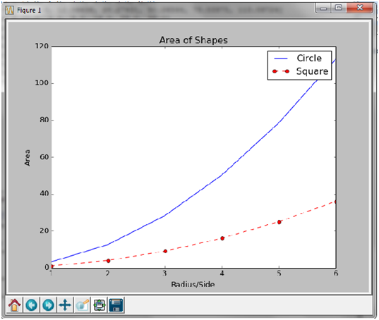
Figure 5. Graph of Area of shapes
Source Code
File Name: plotting.py
from matplotlib import pyplot
from numpy import arange
import bisect
def scatterplot(x, y):
pyplot.plot(x,y,'b.')
pyplot.xlim(min(x)-1, max(x) +1)
pyplot.ylim(min(y)-1, max(y) +1)
pyplot.show ()
def barplot(labels,data):
pos=arange(len (data))
pyplot.xticks(pos+0.4,labels)
pyplot.bar(pos,data)
pyplot.show()
def histplot(data,bins=None,nbins=5):
if not bins:
minx,maxx=min(data),max(data)
space=(maxx-minx)/float(nbins)
bins=arange(minx,maxx,space)
binned=[bisect.bisect(bins,x) for x
in data]
l=['%.1f'%x for x in list(bins)+[maxx]] if space<1 else [str(int(x))
for x in list(bins)+[maxx]]
displab=[x+'-'+y for x,y in
zip(l[:-1],l[1:])]
barplot(displab,[binned.count(x+1)
for x in range(len(bins))])
defbarchart(x,y,numbins=5):
datarange=max(x)-min(x)
bin_width=float(datarange)/numbins
pos=min(x)
bins=[0 for i in range(numbins+1)]
fori in range(numbins):
bins[i]=pos
pos+=bin_width
bins[numbins]=max(x)+1
binsum=[0 for i in range(numbins)]
bincount=[0 for i in
range(numbins)]
binaverage=[0 for i in
range(numbins)]
fori in range(numbins):
for j in range(len(x)):
if x[j]>=bins[i] and
x[j]<bins[i+1]:
bincount[i]+=1
binsum[i]+=y[j]
for i in range(numbins):
binaverage[i]=float(binsum[i])/bincount[i]
barplot(range(numbins),binaverage)
defpiechart(labels,data):
fig=pyplot.figure(figsize=(7,7))
pyplot.pie(data,labels=labels,autopct='%1.2f%%')
pyplot.show()
Using the Wrapper
To use the
wrapper in local environment, simply create a file named plotting.py, copy and
paste the contents of the source code above to it and save it in the work
directory (where it keeps Python code). Alternatively it can modify the PYTHONPATH
environment variable of the Operating System to include the directory where the
wrapper is located.
from plotting import *
barchart ([1, 2, 3, 4, 5], [1, 2,
3, 4, 5],5)

Figure 6. Plotting an array
in bar chart
Source Code
File Name: udacilplt.py
Import matplotlib,
matplotlib.pyplot
import numpy
import types
def show_plot(arg1, arg2=None):
def real_decorator(f):
def wrapper(*args, **kwargs):
matplotlib.pyplot.figure(figsize=(arg1,
arg2))
result = f(*args, **kwargs)
matplotlib.pyplot.show()
return result
return wrapper
if type(arg1) ==
types.FunctionType:
f = arg1
arg1, arg2 = 10, 5
return real_decorator(f)
return real_decorator
code :
import math
from udacilplt import *
@show_plot
def simple():
x_data = numpy.linspace(0., 100.,
1000)
for x in x_data:
y = math.sqrt(x)
matplotlib.pyplot.scatter(x, y)
axes = matplotlib.pyplot.gca()
axes.set_xlabel('x')
axes.set_ylabel('y')
simple()

Figure 7: Plots square root function from 0 to 100
Although it is
possible to create nice bar plots, pie charts, scatter plots, etc., only a few
commands are needed for most computer vision purposes. Most importantly, we
want to be able to show things like interest points, correspondences, and
detected objects using points and lines. The below code is used to plotting an
image with a few points and a line:
Code: plot the
points plot(x,y)
from PIL import
Image
frompylab import
*
im =
array(Image.open('emp.jpg'))
# plot the image
imshow(im)
# some points
x =
[100,100,400,400]
y =
[200,500,200,500]
# plot the
points
plot(x,y)
# line plot
connecting the first two points
plot(x[:2],y[:2])
# add title and
show the plot
title('Plotting:
"emp.jpg"')
show()

Figure 8 . Plot the points
plot(x,y)
Code: plot the points with red star-markers
from PIL import
Image
frompylab import
*
# read image to
array
im =
array(Image.open('emp.jpg'))
# plot the image
# some points
x =
[100,100,400,400]
y =
[200,500,200,500]
# plot the
points with red star-markers
plot(x,y,'r*')
# line plot
connecting the first two points
plot(x[:2],y[:2])
# add title and
show the plot
title('Plotting:
"emp.jpg"')
show()

Figure 9 . Plot the points with red star-markers
Code:
To interact with an application, for
example by marking points in an image, or it need to annotate some training
data.
PyLab comes with a simple function, ginput().
from PIL import
Image
frompylab import
*
im =
array(Image.open('emp.jpg'))
imshow(im)
print 'Please
click 3 points'
x = ginput(3)
print 'you
clicked:',x
show()
Code: Image
Contours and Histograms
from PIL import Image
frompylab import *
# read image to array
im =
array(Image.open('emp.jpg').convert('L'))
# create a new figure
figure()
# don't use colors
gray()
# show contours with origin upper
left corner
contour(im, origin='image')
axis('equal')
axis('off')
figure()
hist(im.flatten(),128)
show()
Code:
The axes are useful for debugging.
from PIL import
Image
frompylab import
*
# read image to
array
im =
array(Image.open('emp.jpg'))
# plot the image
imshow(im)
# some points
x =
[100,100,400,400]
y =
[200,500,200,500]
# plot the
points with red star-markers
plot(x,y,'r*')
# line plot
connecting the first two points
plot(x[:2],y[:2])
axis('off')
# add title and
show the plot
title('Plotting:
"empire.jpg"')
show()
Chapter 4
Filters
They are
algorithms for filtering. Composed of Window mask / Kernel /
Convolution mask and Constants
Convolution (FilteringTechnique)
Process of evaluating the
weighted neighboring pixel values located in a particular spatial pattern
around the i,j, location in input image. The techniques involves a series of
steps:
1. Mask window is placed
over part of image.
2. Convolution Formula is
applied over the part of image (Sum of the Weighted product is obtained
(coefficient of mask x raw DN value)/ sum of coefficients)
3.Central value replaced
by the output value. Window shifted by one pixel & procedure is
repeated for the entire image.
To start with
some image processing, let us make a ‘negative’ of the image ‘scenery’.

Figure10.Negative of a scenery
Filtering
techniques can be done by using Python in-built classes. First of all import
modules - Image, ImageChops, and ImageFilter. After opening the image in
python, by ‘Image.open’ method , we can use different Filters - BLUR Filter,
EMBOSS Filter, CONTOUR filter, Find Edges Filter
etc.
Image Filtering
Using Open Source Software (Python)

Figure11. Original Image of coins
Basic code:
from PIL import
Image, ImageFilter
image =
Image.open('coin.jpg')
image =
image.filter(ImageFilter.FIND_EDGES)
image.save('coins.jpg')
Output:

Figure 12. Filtered Image of a coin to find edges
Code:
importnumpy
importscipy
fromscipy import
ndimage
im = scipy.misc.imread('coin.jpg')
im =
im.astype('int32')
dx =
ndimage.sobel(im, 0)
dy =
ndimage.sobel(im, 1)
mag =
numpy.hypot(dx, dy)
mag *= 255.0 /
numpy.max(mag)
scipy.misc.imsave('sobel1.jpg',
mag)
Output :

Figure 13. Filtered sobel
image
High Pass Filtering
"High pass filter" is a very
generic term. There are an infinite number of different "highpass
filters" that do very different things (e.g. an edge dectection filter, as
mentioned earlier, is technically a highpass (i.e. most are actually a
bandpass) filter, but has a very different effect from what probably had in
mind.)
High Pass
Filtering is applied to imagery to remove the slowly varying components and
enhance the high frequency local variations. One high frequency filter
(HFF5,out) is computed by subtracting the output of the low frequency filter
(LFF5,out) from twice the value of the original central pixel value.The salient
features of High Pass Filters
·
Preserves high frequencies and Removes slowly
varying components
·
Emphasizes fine details
·
Used for edge detection and enhancement
·
Edges - Locations where transition from one
category to other occurs
Brightness
values tend to be highly correlated in a nine element window. Thus, the high
frequency or high pass filtered image will have a relatively narrow intensity
histogram. This suggests that the output from most high frequency filtered
images must be contrast stretched prior to visual analysis. High pass filtering
is used for edge enhancement.
import matplotlib.pyplot as plt
import numpy as np
from scipy import ndimage
import Image
def plot(data, title):
plot.i += 1
plt.subplot(2,2,plot.i)
plt.imshow(data)
plt.gray()
plt.title(title)
plot.i = 0
# Load the data...
im = Image.open('abc.png')
data = np.array(im, dtype=float)
plot(data, 'Original')
# A very simple and very narrow
highpass filter
kernel = np.array([[-1, -1, -1],
[-1, 8, -1],
[-1, -1, -1]])
highpass_3x3 =
ndimage.convolve(data, kernel)
plot(highpass_3x3, 'Simple 3x3
Highpass')
# A slightly "wider", but
sill very simple highpass filter
kernel = np.array([[-1, -1, -1, -1,
-1],
[-1, 1,
2, 1, -1],
[-1, 2,
4, 2, -1],
[-1, 1,
2, 1, -1],
[-1, -1, -1, -1, -1]])
highpass_5x5 = ndimage.convolve(data,
kernel)
plot(highpass_5x5, 'Simple 5x5
Highpass')
# Another way of making a highpass
filter is to simply subtract a lowpass
# filtered
image from the original. Here, we'll use a simple gaussian filter
# to "blur" (i.e. a
lowpass filter) the original.
lowpass =
ndimage.gaussian_filter(data, 3)
gauss_highpass = data - lowpass
plot(gauss_highpass,
r'GaussianHighpass, $\sigma = 3 pixels$')
plt.show()

Figure 14. Original image
Chapter 5
Python Patterns: Crop Images with PIL/Pillow
Cropping refers
to the removal of the outer parts of an image to improve framing, accentuate
subject matter or change aspect ratio. Depending on the application, this may
be performed on a physical photograph, artwork, film footage, or achieved
digitally using any programming language.
In the printing,
graphic design and photography industries, cropping plays very important role
to remove unwanted areas from the photographic to illustrated image. One of the
most basic photo manipulation processes, it is performed in order to remove an
unwanted subject or irrelevant details from photo, change its aspect ratio, or
to improve overall composition.
There are many
reasons to crop an image; for example fitting an image to the fill a frame, removing
a portion of the background to emphasize the subject, etc.
There are some
methods to crop an image :
·
Crop image from top-left corner
|
·
Crop image from bottom-right corner
|
·
Crop image starting in the center
·
Adjust image in the area from starting
·
Pad the image to a square
|
crop.py
# Import Pillow
from PIL import Image
# Load the original image:
img =
Image.open("flower.jpg")
#100px * 100px, starting at the
top-left corner
img2 = img.crop((0, 0, 500, 500))
img2.save("img_2.jpg")
#500px * 500px, starting at the
bottom-right corner
width = img.size[0]
height = img.size[1]
img3 = img.crop(
(
width - 500,
height - 500,
width,
height
)
)
img3.save("img_3.jpg")
#starting in the center
half_the_width = img.size[0] / 2
half_the_height = img.size[1] / 2
img4 = img.crop(
(
half_the_width - 500,
half_the_height - 750,
half_the_width + 500,
half_the_height + 750
)
)
img4.save("img_4.jpg")
#starting
half_the_width = img.size[0] / 2
half_the_height = img.size[1] / 2
img4 = img.crop(
(
half_the_width - 750,
half_the_height - 550,
half_the_width + 750,
half_the_height + 550
)
)
img4.save("img_5.jpg")
#Pad the image to a square
longer_side = max(img.size)
horizontal_padding = (longer_side -
img.size[0]) / 2
vertical_padding = (longer_side -
img.size[1]) / 2
img5 = img.crop(
(
-horizontal_padding,
-vertical_padding,
img.size[0] + horizontal_padding,
img.size[1] + vertical_padding
)
)
img5.save("img_6.jpg")
Chapter 6
Python
Patterns: Rotate Images with PIL/Pillow
The Image module
provides the class with the same name which is used to present PIL image. The
module also provides a number of factory functions, including functions to load
images from files, and to create new images.
The following
script loads an image, rotates it counter clockwise rotation and clockwise
rotation by the specified number of degrees. and displays it using an external
viewer. The image shown rotated and then saved to the working folder. PIL
handles a fair amount of image file formats easily.
Types of
rotation of images are as follows :
·
Counterclockwise Rotation
·
Clockwise Rotation
Counterclockwise Rotation: A
counterclockwise rotation is one that proceeds in the opposite direction , from
the top to the left, then down and then to the right, and back up to the top.
·
Rotate counterclockwise 900
·
Rotate counterclockwise 450
Clockwise Rotation: A clockwise rotation is one that proceeds in the same direction as a clock's hands, from the
top to the right, then down and then to the left, and back up to the top.
·
Rotate clockwise 900
·
Rotate clockwise 450
# Import Pillow:
from PIL import Image
# Load the original image:
img =
Image.open("flower.jpg")
#Counterclockwise Rotation
img22 = img.rotate(45)
img22.save("img22.jpg")
img32 = img.rotate(90)
img32.save("img32.jpg")
#Clockwise Rotation
img42 = img.rotate(-45)
img42.save("img42.jpg")
#Disable cropping of the output
image
img52 = img.rotate(45, expand=True)
img52.save("img52.jpg")
#Apply a resampling filter
# Nearest neighbor (default):
img62 = img.rotate(45,
resample=Image.NEAREST)
img62.save("img62.jpg")
# Linear interpolation:
img72 = img.rotate(45,
resample=Image.BILINEAR)
img72.save("img72.jpg")
# Cubic spline interpolation:
img82 = img.rotate(45,
resample=Image.BICUBIC)
img82.save("img82.jpg")
Code:
import Image, math
deffind_centroid(im):
width, height = im.size
XX, YY, count = 0, 0, 0
for x in xrange(0, width, 1):
for y in xrange(0, height, 1):
ifim.getpixel((x, y)) == 0:
XX += x
YY += y
count += 1
return XX/count, YY/count
#Top Left Vertex
def find_vertex1(im):
width, height = im.size
for y in xrange(0, height, 1):
for x in xrange (0, width, 1):
ifim.getpixel((x, y)) == 0:
X1=x
Y1=y
return X1, Y1
#Bottom Left Vertex
def find_vertex2(im):
width, height = im.size
for x in xrange(0, width, 1):
for y in xrange (height-1, 0, -1):
ifim.getpixel((x, y)) == 0:
X2=x
Y2=y
return X2, Y2
#Top Right Vertex
def find_vertex3(im):
width, height = im.size
for x in xrange(width-1, 0, -1):
for y in xrange (0, height, 1):
ifim.getpixel((x, y)) == 0:
X3=x
Y3=y
return X3, Y3
#Bottom Right Vertex
def find_vertex4 (im):
width, height = im.size
for y in xrange(height-1, 0, -1):
for x in xrange (width-1, 0, -1):
ifim.getpixel((x, y)) == 0:
X4=x
Y4=y
return X4, Y4
deffind_angle (V1, V2, direction):
side1=math.sqrt(((V1[0]-V2[0])**2))
side2=math.sqrt(((V1[1]-V2[1])**2))
if direction == 0:
returnmath.degrees(math.atan(side2/side1)),
'Clockwise'
return 90-math.degrees(math.atan(side2/side1)),
'Counter Clockwise'
#Find direction of Rotation; 0 =
CW, 1 = CCW
deffind_direction (vertices, C):
high=480
for i in range (0,4):
if vertices[i][1]<high:
high = vertices[i][1]
index = i
if vertices[index][0]<C[0]:
return 0
return 1
def main():
im = Image.open('p.jpg')
im = im.convert('1') # convert
image to black and white
print 'Centroid ',
find_centroid(im)
print 'Top Left ', find_vertex1
(im)
print 'Bottom Left ', find_vertex2
(im)
print 'Top Right', find_vertex3
(im)
print 'Bottom Right ', find_vertex4
(im)
C = find_centroid (im)
V1 = find_vertex1 (im)
V2 = find_vertex3 (im)
V3 = find_vertex2 (im)
V4 = find_vertex4 (im)
vertices = [V1,V2,V3,V4]
direction =
find_direction(vertices, C)
print 'angle: ', find_angle(V1,V2,direction)
if __name__ == '__main__':
main()
Some more observations regarding
image processing :
importnumpy as np
importscipy
fromscipy import ndimage
im =
scipy.misc.imread('empirestate.jpg',flatten=1)
im = np.where(im> 128, 0, 1)
label_im, num = ndimage.label(im)
slices =
ndimage.find_objects(label_im)
centroids =
ndimage.measurements.center_of_mass(im, label_im, xrange(1,num+1))
angles = []
for s in slices:
height, width = label_im[s].shape
opp = height - np.where(im[s][:,-1]==1)[0][-1]
- 1
adj = width -
np.where(im[s][-1,:]==1)[0][0] - 1
angles.append(np.degrees(np.arctan2(opp,adj)))
print 'centers:', centroids
print 'angles:', angles
print im
Chapter 7
Edge Detection
Edge detection
is one of the fundamental operations when we perform image processing. It helps
us reduce the amount of datato process and maintains the structural aspect of
the image. We are going to look into commonly used edge detection schemes-
gradient(sobel-first order derivative) based edge detector. It work with
convolutions and achieve the same end goal Edge Detection.
Sobel edge
detector is a gradient based method based on the first order derivatives.
Edge detection aim at identifying points
in a digital image at
which the image
brightness changes sharply or, more formally, has discontinuities.
The points at which image brightness changes sharply are typically organized
into a set of curved line segments termed edges. The same problem of finding discontinuities in 1D
signals is known as step
detection and the problem of finding signal discontinuities over
time is known as change
detection. Edge detection is a fundamental tool in image processing, machine vision and computer vision,
particularly in the areas of feature
detection and feature
extraction.
The purpose of
detecting sharp changes in image brightness is to capture important events and
changes in properties of the world. It can be shown that under rather general
assumptions for an image formation model, discontinuities in image brightness
are likely to correspond to:
·
discontinuities in depth,
·
discontinuities in surface orientation,
·
changes in material properties and
·
variations in scene illumination.
Edges extracted
from non-trivial images are often hampered by fragmentation, meaning that the edge curves are not
connected, missing edge segments as well as false edges not
corresponding to interesting phenomena in the image – thus complicating the
subsequent task of interpreting the image data.
Edge detection
is one of the fundamental steps in image processing, image analysis, image
pattern recognition, and computer vision techniques.
Although certain
literature has considered the detection of ideal step edges, the edges obtained
from natural images are usually not at all ideal step edges. Instead they are
normally affected by one or several of the following effects:
·
focal blur caused by a finite depth-of-field and finite point spread function.
·
penumbral blur caused by shadows created by light sources of non-zero
radius.
·
shading at a smooth object
A number of
researchers have used a Gaussian smoothed step edge (an error function) as the
simplest extension of the ideal step edge model for modeling the effects of
edge blur in practical applications. Thus,
a one-dimensional image
which
has exactly one edge placed at
may
be modeled as:
At the left side
of the edge, the intensity is
, and right of the edge it is
. The scale parameter
is
called the blur scale of the edge.
PIL has a find edges method that gives an image of just the
edges:

Figure 15.
Image ofAlbino
from PIL import Image, ImageFilter
im = Image.open('albino.jpg')
im1 =
im.filter(ImageFilter.FIND_EDGES)
im1 = im1.convert('1')
print im1
im1.save("EDGES.jpg")
Output:

Figure 16 . Finding Edgesof Albino
Non Linear Edge
Enhancement
Non linear edge enhancement are
performed using nonlinear combinations of pixels. Many algorithms are applied
using either 2 x 2 of 3 x3 kernels.

Figure 17 . Input image for Edge Enhancement
import numpy
import scipy
from scipy import ndimage
im = scipy.misc.imread('deep.jpg')
im = im.astype('int32')
dx = ndimage.sobel(im, 1) # horizontal derivative
dy = ndimage.sobel(im, 0) # vertical derivative
mag = numpy.hypot(dx, dy) # magnitude
mag *= 255.0 / numpy.max(mag) # normalize (Q&D)
scipy.misc.imsave('sobel.jpg', mag)
Output :

Figure 18 .Sobel Image
Chapter
8
Piecewise Linear
Stretch
When
the distribution of a histogram in an image is bi or tri-modal, an analyst may
stretch certain values of the histogram for increased enhancement in selected
areas. This method of contrast enhancement is called a piecewise linear
contrast stretch. A piecewise linear contrast enhancement involves the
identification of a number of linear enhancement steps that expands the
brightness ranges in the modes of the histogram.
In
the piecewise stretch, a series of small min-max stretches are set up within a
single histogram.
The piecewise linear enhancement
gives a much better result than the linear enhancement when data exhibits
multi-modal distribution across the histogram of data values, which was a major
limitation for linear enhancement. The cost of this transformation is that the
linear relation between the input and output pixel values is lost.
This figure was
obtained by setting on the lines. I attempted to apply a piecewise linear fit
using the code:
from scipy import optimize
import matplotlib.pyplot as plt
import numpy as np
x = np.array([1, 2, 3, 4, 5, 6, 7,
8, 9, 10 ,11, 12, 13, 14, 15])
y = np.array([5, 7, 9, 11, 13, 15,
28.92, 42.81, 56.7, 70.59, 84.47, 98.36, 112.25, 126.14, 140.03])
defline ar_fit(x, a, b):
return a * x + b
fit_a, fit_b =
optimize.curve_fit(linear_fit, x[0:5], y[0:5])[0]
y_fit = fit_a * x[0:7] + fit_b
fit_a, fit_b =
optimize.curve_fit(linear_fit, x[6:14], y[6:14])[0]
y_fit = np.append(y_fit, fit_a *
x[6:14] + fit_b)
figure = plt.figure(figsize=(5.15,
5.15))
figure.clf()
plot = plt.subplot(111)
ax1 = plt.gca()
plot.plot(x, y, linestyle = '',
linewidth = 0.25, markeredgecolor='none', marker = 'o', label =
r'\textit{y_a}')
plot.plot(x, y_fit, linestyle =
':', linewidth = 0.25, markeredgecolor='none', marker = '', label =
r'\textit{y_b}')
plot.set_ylabel('Y', labelpad = 6)
plot.set_xlabel('X', labelpad = 6)
figure.savefig('test.pdf',
box_inches='tight')
plt.close()
Result:

Figure 19 . Piecewise linear fit
Useof numpy.piecewise() is to
create the piecewise function and then use curve_fit(), Here is the code:
from scipy import optimize
import matplotlib.pyplot as plt
import numpy as np
x = np.array([1, 2, 3, 4, 5, 6, 7,
8, 9, 10 ,11, 12, 13, 14, 15], dtype=float)
y = np.array([5, 7, 9, 11, 13, 15,
28.92, 42.81, 56.7, 70.59, 84.47, 98.36, 112.25, 126.14, 140.03])
defpiecewise_linear(x, x0, y0, k1,
k2):
returnnp.piecewise(x, [x < x0],
[lambda x:k1*x + y0-k1*x0, lambda x:k2*x + y0-k2*x0])
figure = plt.figure(figsize=(5.15,
5.15))
figure.clf()
plot = plt.subplot(111)
p , e =
optimize.curve_fit(piecewise_linear, x, y)
xd = np.linspace(0, 15, 100)
plot.plot(x, y, "o")
plot.plot(xd, piecewise_linear(xd,
*p))
figure.savefig('deep.pdf',box_inches='tight')
plt.close()
Result :

Figure 20. Curve_fitfunction
to plot Piecewise linear
Spline
interpolation schemeis
used toperform piecewise linear interpolation and
find the turning point of the curve. The second derivative will be the highest
at the turning point (for an monotonically increasing curve), and can be
calculated with a spline interpolation of order > 2.
import numpy as
np
import matplotlib.pyplot as plt
from scipy import interpolate
x = np.array([1, 2, 3, 4, 5, 6, 7,
8, 9, 10 ,11, 12, 13, 14, 15])
y = np.array([5, 7, 9, 11, 13, 15,
28.92, 42.81, 56.7, 70.59, 84.47, 98.36, 112.25, 126.14, 140.03])
tck = interpolate.splrep(x, y, k=2,
s=0)
xnew = np.linspace(0, 15)
fig, axes = plt.subplots(3)
axes[0].plot(x, y, 'x', label =
'data')
axes[0].plot(xnew,
interpolate.splev(xnew, tck, der=0), label = 'Fit')
axes[1].plot(x,
interpolate.splev(x, tck, der=1), label = '1st dev')
dev_2 = interpolate.splev(x, tck,
der=2)
axes[2].plot(x, dev_2, label = '2st
dev')
turning_point_mask = dev_2 ==
np.amax(dev_2)
axes[2].plot(x[turning_point_mask],
dev_2[turning_point_mask],'rx',
label = 'Turning point')
for ax in axes:
ax.legend(loc = 'best')
plt.show()
Result :

Figure 21 Turning point fit using spline interpolation
FUTURE WORK
1.
Artificial Neural Networks (ANN) as mathematical models
for back-propagation learning and classification of Remote Sensing Images.
2.
Neural Networks will be used
3.
Broader File Format Supports:
a.
The Current implementation of the software supports
common image formats like JPEG, GIF, PNG, TIFF (Tagged Image File Format)
b.
Satellites use multiple formats for data compression,
and lossless recovery – like MODIS, HRPT, CZCS, Dundee, HDF, etc.
4.
Parallel Batch Processing of Data
5.
Licensing
a.
Since the code is open source in nature, it must comply
with the FOSS (Free and Open Source Software) standards.
b.
The options of licenses, recognized by the Open Source
Initiative
6.
One of the things we could do to make edge detection
algorithm better would be to develop a more optimal edge detection scheme that
leaves thinner edges than the gradient detector used but also would be more
resistant to noise than a Laplacian edge detector. One possibility would be to
implement a multiscale edge detector to solve that problem. Another improvement
would be to find a better thresholding scheme than setting a range that the
number of `edge' pixels has to fall into. Again, the multiscale edge detector
might eliminate the need for much thresholding.
CONCLUSION
a.
scipy
b.
PIL/pillow
c.
matplotlib
d.
tkinter
e.
numpy
f.
scikit
g.
scikit-learn
2.
The present supports JPEG, GIF, PNG, file import. This
covers 30% of the satellite image formats.
3.
Enhancement features currently supported are –
Contrast, Spectral, and Spatial.
4.
The Machine Learning Algorithms currently supported
are:
a.
Supervised learning which utilizes the spectral Python
library.
b.
Unsupervised Learning
5.
A key benefit of edge detection technique is that it
responds strongly to Mach
bands, and avoids false positives typically found around roof edges. A roof edge,
is a discontinuity in the first order derivative of a grey-level profile.
6.
Edge detection technique is used in image processing, machine vision and computer vision,
particularly in the areas of feature
detection and feature
extraction.
REFERENCES
- https://onlinecourses.science.psu.edu/stat857/book/export/html/11
- http://courses.edx.org/
- Umbaugh, Scott E (2010). Digital image processing and analysis : human and computer vision applications with CVIPtools (2nd ed. ed.). Boca Raton, FL: CRC Press. ISBN 9-7814-3980-2052. http://stat.ethz.ch/~maathuis/teaching/fall08/Notes3.pdf
- http://compdiag.molgen.mpg.de/ngfn/docs/2003/nov/svm.pdf
- http://en.wikipedia.org/wiki/Support_vector_machine
- http://matplotlib.org/users/pyplot
- http://plot.ly/python/line-and-scatter-plots-tutorial
- www.owlnet.rice.edu/~elec539/Projects97/morphjrks/moredge.html
- www.cse.unr.edu.html/~bebis/CS791E/Notes/EdgeDetection.pdf
- www.mathworks.com/discovery/edge-detection
- http://www.engpaper.com/image-processing-research-paper-51.htm
- http://docs.gimp.org/2.6/en/gimp-layer-rotate-270.html
- N. Nacereddine, L. Hamami, M. Tridi, and N. Oucief , “Non-Parametric Histogram-Based Thresholding Methods for Weld Defect Detection in Radiography “ ,online access
- Gerhard X. Ritter; Joseph N. Wilson, “Handbook of Computer Vision Algorithms in Image
Algebra” CRC Press, CRC Press LLC ISBN: 0849326362 Pub Date: 05/01/96
- http://www.engpaper.com/image-processing-research-paper-51.htm
- www.google.com
- https://www.wikipedia.org/


Comments